thztools.noisefit#

thztools.noisefit(x, *, dt=None, sigma_alpha0=None, sigma_beta0=None, sigma_tau0=None, mu0=None, a0=None, eta0=None, fix_sigma_alpha=False, fix_sigma_beta=False, fix_sigma_tau=False, fix_mu=False, fix_a=False, fix_eta=False, scale_logv_alpha=None, scale_logv_beta=None, scale_logv_tau=None, scale_delta_mu=None, scale_delta_a=None, scale_eta=None, min_options=None)[source]#

Estimate noise model from a set of nominally identical waveforms.

The data array x should include m nominally identical waveform measurements, where each waveform comprises n samples that are spaced equally in time. The noise_model attribute of the return object is an instance of the NoiseModel class that represents the estimated noise parameters. See Notes for details.

Parameters:

xarray_like with shape (n, m): Data array composed of m waveforms, each of which is sampled at n points.
dtfloat or None, optional: Sampling time, normally in picoseconds. Default is None, which sets the sampling time to thztools.options.sampling_time. If both dt and thztools.options.sampling_time are None, the sampling time is set to 1.0. In this case, the unit of time is the sampling time for the noise model parameter sigma_tau, the delay parameter array eta, and the initial guesses for both quantities.
sigma_alpha0, sigma_beta0, sigma_tau0float, optional: Initial values for noise parameters. When set to None, the default, use a linear least-squares fit of the noise model to np.var(x, 1, ddof=1).
mu0array_like with shape(n,), optional: Initial guess, signal vector with shape (n,). Default is first column of x.
a0array_like with shape(m,), optional: Initial guess, signal amplitude drift vector with shape (m,). Default is np.ones(m).
eta0array_like with shape(m,), optional: Initial guess, signal delay drift vector with shape (m,). Default is np.zeros(m).
fix_sigma_alpha, fix_sigma_beta, fix_sigma_taubool, optional: Fix the associated noise parameter. Default is False.
fix_mubool, optional: Fix signal vector. Default is False.
fix_abool, optional: Fix signal amplitude drift vector. Default is False.
fix_etabool, optional: Fix signal delay drift vector. Default is False.

Returns:

resNoiseResult: Fit result represented as a NoiseResult object. Important attributes are: noise_model, an instance of NoiseModel with the estimated noise parameters; mu, the estimated signal vector; a, the estimated signal amplitude drift vector; eta, the estimated signal delay drift vector; fval, the value of the optimized NLL cost function; and diagnostic, an instance of scipy.optimize.OptimizeResult returned by scipy.optimize.minimize. Note that the fit parameters are scaled internally to improve convergence (see Other Parameters below), which affects the attributes fun, jac, and hess_inv of diagnostic. See NoiseResult for more details and for a description of other attributes.

Other Parameters:

scale_logv_alpha, scale_logv_beta, scale_logv_taufloat, optional: Scale for varying the log of the variance parameters.
scale_delta_muarray_like with shape(n,), optional: Scale for varying signal vector. When set to None, the default, use NoiseModel(sigma_alpha0, sigma_beta0, sigma_tau0).noise_amp(mu0).
scale_delta_aarray_like with shape(n,), optional: Scale for varying signal amplitude drift vector. Default is np.max((sigma_min, sigma_beta0)) for all entries, where sigma_min = np.sqrt(np.min(np.var(x, 1, ddof=1))).
scale_etaarray_like with shape(n,), optional: Scale for varying signal delay drift vector. Default is np.max((sigma_min, sigma_tau0)), for all entries, where sigma_min = np.sqrt(np.min(np.var(x, 1, ddof=1))).
min_optionsdict or None, optional: Keyword options passed to the options parameter of scipy.optimize.minimize. See the documentation on the BFGS method for details. By default, gtol=1e-5 * x.size. The options eps and finite_diff_rel_step are not used.

Raises:

ValueError: If all parameters are held fixed or if the input arrays have incompatible shapes.

Warns:

UserWarning: If thztools.options.sampling_time and the dt parameter are both not None and are set to different float values, the function will set the sampling time to dt and raise a UserWarning.

See also

NoiseModel: Noise model class.

Notes

Given an \(N\times M\) data array \(\mathbf{X}\), the function uses the BFGS method of scipy.optimize.minimize to minimize the maximum-likelihood cost function [1]

\[\begin{split}\ Q_\text{ML}\ (\sigma_\alpha,\sigma_\beta,\sigma_\tau,\boldsymbol{\mu},\ \mathbf{A},\boldsymbol{\eta};\mathbf{X})\ = \frac{1}{2}\sum_{k=0}^{N-1}\sum_{l=0}^{M-1}& \ \left[\ln\sigma_{kl}^2 + \frac{(X_{kl} \ - Z_{kl})^2}{\sigma_{kl}^2}\right]\ \end{split}\]

with respect to the unknown model parameters \(\sigma_\alpha\), \(\sigma_\beta\), \(\sigma_\tau\), \(\boldsymbol{\mu}\), \(\mathbf{A}\) and \(\boldsymbol{\eta}\). The model assumes that the elements of \(\mathbf{X}\) are normally distributed around the corresponding elements of \(\mathbf{Z}\) with variances given by \(\boldsymbol{\sigma}^2\), which are in turn given by

\[Z_{kl} = A_l\mu(t_k - \eta_l)\]

and

\[\sigma_{kl}^2 = \sigma_\alpha^2 + \sigma_\beta^2 Z_{kl}^2 \ + \sigma_\tau^2(\mathbf{D}\mathbf{Z})_{kl}^2,\]

where \(\mathbf{D}\) is the time-domain derivative operator. The function \(\mu(t)\) represents an ideal primary waveform, which drifts in amplitude and temporal location between each of the \(M\) waveform measurements. Each waveform comprises \(N\) samples at the nominal times \(t_k\), and the drift in the amplitude and the temporal location of the \(l\) waveform are given by \(A_l\) and \(\eta_l\), respectively, with initial values fixed at \(A_0 = 1.0\) and \(\eta_0 = 0.0\) by definition.

References

[1]

Laleh Mohtashemi, Paul Westlund, Derek G. Sahota, Graham B. Lea, Ian Bushfield, Payam Mousavi, and J. Steven Dodge, “Maximum- likelihood parameter estimation in terahertz time-domain spectroscopy,” Opt. Express 29, 4912-4926 (2021), https://doi.org/10.1364/OE.417724.

Examples

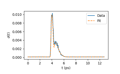
In basic usage, it should be possible to call noisefit with just the data array. In the code below, we simulate m = 50 noisy waveforms with n = 256 time points each, then verify that the fit results are consistent with the true noise parameters.

>>> import numpy as np
>>> import thztools as thz
>>> from matplotlib import pyplot as plt
>>> rng = np.random.default_rng(0)
>>> n, m, dt = 256, 50, 0.05
>>> t = thz.timebase(n, dt=dt)
>>> mu = thz.wave(n, dt=dt)
>>> alpha, beta, tau = 1e-4, 1e-2, 1e-3
>>> noise_model = thz.NoiseModel(sigma_alpha=alpha, sigma_beta=beta,
...  sigma_tau=tau, dt=dt)
>>> a = 1.0 + 1e-2 * np.concatenate(([0.0],
...                                 rng.standard_normal(m - 1)))
>>> eta = 1e-3 * np.concatenate(([0.0], rng.standard_normal(m - 1)))
>>> z = thz.scaleshift(np.repeat(np.atleast_2d(mu), m, axis=0), dt=dt,
...                    a=a, eta=eta).T  # Orient the array columnwise
>>> x = z + noise_model.noise_sim(z, axis=0, seed=12345)
>>> noise_res = thz.noisefit(x, sigma_alpha0=alpha, sigma_beta0=beta,
...  sigma_tau0=tau, dt=dt)
>>> noise_res.noise_model
NoiseModel(sigma_alpha=0.000100..., sigma_beta=0.00984...,
sigma_tau=0.000899..., dt=0.05)

>>> plt.plot(t, np.std(thz.scaleshift(x, a=1 / noise_res.a,
... eta=-noise_res.eta, axis=0), axis=1), "-",
... label="Data")
>>> plt.plot(t, noise_res.noise_model.noise_amp(noise_res.mu),
...  "--", label="Fit")
>>> plt.legend()
>>> plt.xlabel("t (ps)")
>>> plt.ylabel(r"$\sigma(t)$")
>>> plt.show()