thztools.apply_frf

thztools.apply_frf(frfun, x, *, dt=None, numpy_sign_convention=True, args=())

Apply a frequency response function to a waveform.

Parameters:

frfuncallable

Frequency response function.

frfun(omega, *args) -> ndarray

where omega is an array of angular frequencies and args is a tuple of the fixed parameters needed to completely specify the function. The units of omega must be the inverse of the units of dt, such as radians/picosecond.

xarray_like

Data array.

dtfloat or None, optional

Sampling time, normally in picoseconds. Default is None, which sets the sampling time to thztools.options.sampling_time. If both dt and thztools.options.sampling_time are None, the sampling time is set to 1.0. In this case, the angular frequency omega must be given in units of radians per sampling time, and any parameters in args must be expressed with the sampling time as the unit of time.

numpy_sign_conventionbool, optional

Adopt NumPy sign convention for harmonic time dependence, e.g., express a harmonic function with frequency \(\omega\) as \(x(t) = a e^{i\omega t}\). Default is True. When set to False, uses the convention more common in physics, \(x(t) = a e^{-i\omega t}\).

argsarray_like, optional

Extra arguments passed to the frequency response function. All elements must be real quantities.

Returns:

yndarray

Result of applying the frequency response function to x.

Warns:

UserWarning

If thztools.options.sampling_time and the dt parameter are both not None and are set to different float values, the function will set the sampling time to dt and raise a UserWarning.

See also

fit

Fit a frequency response function to time-domain data.

Notes

The output waveform is computed by transforming \(x[n]\) into the frequency domain, multiplying by the frequency response function \(H[n]\), then transforming back into the time domain.

\[y[n] = \mathcal{F}^{-1}\{H[n] \mathcal{F}\{x[n]\}\}\]

Examples

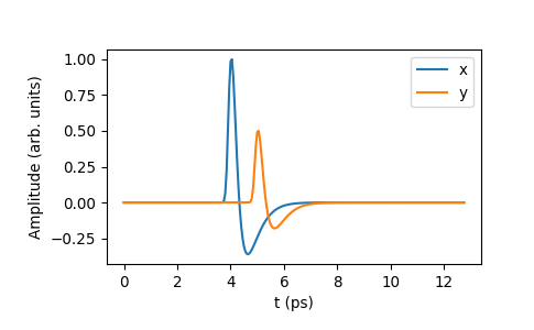
Apply a frequency response function that rescales the input by \(a\) and shifts it by \(\tau\).

\[H(\omega) = a\exp(-i\omega\tau).\]

Note that this form assumes the \(e^{+i\omega t}\) representation of harmonic time dependence, which corresponds to the default setting numpy_sign_convention=True.

>>> import numpy as np
>>> import thztools as thz
>>> from matplotlib import pyplot as plt
>>> n, dt = 256, 0.05
>>> t = thz.timebase(n, dt=dt)
>>> x = thz.wave(n, dt=dt)
>>> def shiftscale(_w, _a, _tau):
...     return _a * np.exp(-1j * _w * _tau)
>>>
>>> y = thz.apply_frf(
...     shiftscale, x, dt=dt, numpy_sign_convention=True, args=(0.5, 1)
... )

>>> _, ax = plt.subplots()
>>>
>>> ax.plot(t, x, label="x")
>>> ax.plot(t, y, label="y")
>>> ax.legend()
>>> ax.set_xlabel("t (ps)")
>>> ax.set_ylabel("Amplitude (arb. units)")
>>> plt.show()

If the frequency response function is expressed using the \(e^{-i\omega t}\) representation more common in physics,

\[H(\omega) = a\exp(i\omega\tau),\]

set numpy_sign_convention=False.

>>> def shiftscale_phys(_w, _a, _tau):
...     return _a * np.exp(1j * _w * _tau)
>>>
>>> y_p = thz.apply_frf(
...     shiftscale_phys, x, dt=dt, numpy_sign_convention=False, args=(0.5, 1)
... )

>>> _, ax = plt.subplots()
>>>
>>> ax.plot(t, x, label="x")
>>> ax.plot(t, y_p, label="y")
>>>
>>> ax.legend()
>>> ax.set_xlabel("t (ps)")
>>> ax.set_ylabel("Amplitude (arb. units)")
>>>
>>> plt.show()