thztools.fit#

thztools.fit(frfun, xdata, ydata, p0, noise_parms=None, *, dt=None, numpy_sign_convention=True, args=(), kwargs=None, f_bounds=None, p_bounds=None, jac=None, lsq_options=None)[source]#

Fit a parameterized frequency response function to time-domain data.

Determines the total least-squares fit to xdata and ydata, given the parameterized frequency response function relationship frfun and noise model parameters noise_parms.

Parameters:

frfuncallable

Frequency response function with signature frfun(omega, *p, *args, **kwargs) that returns an ndarray. Assumes the \(+i\omega t\) convention for harmonic time dependence when numpy_sign_convention is True, the default. All elements of p and args and all values of kwargs must be real quantities.

xdataarray_like

Measured input signal.

ydataarray_like

Measured output signal.

p0array_like

Initial guess for the parameters p.

noise_parmsarray_like or None, optional

Noise parameters (sigma_alpha, sigma_beta, sigma_tau) used to define the :class:NoiseModel for the fit. Default is None, which sets noise_parms to (1.0, 0.0, 0.0).

dtfloat or None, optional

Sampling time, normally in picoseconds. Default is None, which sets dt to thztools.options.sampling_time. If both dt and thztools.options.sampling_time are None, dt is set to 1.0. In this case, the angular frequency omega must be given in units of radians per sampling time, and any parameters in args must be expressed with dt as the unit of time.

numpy_sign_conventionbool, optional

Adopt NumPy sign convention for harmonic time dependence, e.g, express a harmonic function with frequency \(\omega\) as \(x(t) = a e^{i\omega t}\). Default is True. When set to False, uses the convention more common in physics, \(x(t) = a e^{-i\omega t}\).

argstuple

Additional arguments for frfun. All elements must be real.

kwargsdict or None, optional

Additional keyword arguments for frfun. Default is None, which passes no keyword arguments. All values must be real.

f_boundsarray_like, optional

Lower and upper bounds on the frequencies included in the fit. For f_bounds = (f_lo, f_hi), the included frequencies f satisfy

f_lo <= f <= f_hi.

The default is None, which sets f_bounds to include all frequencies except zero:

f_bounds = (np.finfo(np.float64).smallest_normal, np.inf).

Set the lower bound to 0.0 or any negative number to include zero frequency.

p_boundsNone, 2-tuple of array_like, or scipy.optimize.Bounds, optional

Lower and upper bounds on fit parameter(s). Default is None, which sets all parameter bounds to (-np.inf, np.inf). Each bound constraint (p_lo, p_hi) represents a closed interval for the parameter p,

p_lo <= p <= p_hi.

jaccallable or None, optional

Jacobian of the frequency response function with respect to the fit parameters, with signature jac(w, *p, *args, **kwargs). Default is None, which uses scipy.optimize.approx_fprime.

lsq_optionsdict or None, optional

Keyword options passed to scipy.optimize.least_squares. The following keywords are allowed:

“ftol” : Tolerance for termination by the change of the cost function. Default is 1e-8.

“xtol” : Tolerance for termination by the change of the independent variables. Default is 1e-8.

“gtol” : Tolerance for termination by the norm of the gradient. Default is 1e-8.

“loss” : Determines the loss function. Default is “linear”, which gives a standard least-squares problem. Alternative settings have not been tested and should be considered experimental.

“f_scale” : Value of soft margin between inlier and outlier residuals. This parameter has no effect with loss="linear". Default is 1.0.

“max_nfev” : Maximum number of function evaluations before the termination. If None (default), the value is chosen automatically.

“verbose” : Level of algorithm’s verbosity. Default is 0, which works silently.

See the documentation for scipy.optimize.least_squares for details.

Returns:

resFitResult: Fit result represented as a FitResult object. Important attributes are: p_opt, the optimal fit parameter values; p_cov, the parameter covariance matrix estimated from fit; resnorm, the value of the total least-squares cost function for the fit; dof, the number of statistical degrees of freedom in the fit; r_tls, and success, which is True when the fit converges. See the Notes section below and the FitResult documentation for more details and for a description of other attributes.

Raises:

ValueError: If noise_parms does not have 3 elements.

Warns:

UserWarning: If thztools.options.sampling_time and the dt parameter are both not None and are set to different float values, the function will set the sampling time to dt and raise a UserWarning.

See also

NoiseModel: Noise model class.

Notes

This function computes the maximum-likelihood estimate for the parameters \(\boldsymbol{\theta}\) in the frequency response function model \(H(\omega; \boldsymbol{\theta})\) by minimizing the total least-squares cost function

\[Q_\text{TLS}(\boldsymbol{\theta}) \ = \sum_{k=0}^{N-1}\left[ \ \frac{(x_k - \mu_k)^2}{\sigma_{\mathbf{x},k}^2} \ + \frac{(y_k - \psi_k)^2}{\sigma_{\mathbf{y},k}^2} \ \right],\]

where \(\mathbf{x}\) is the input signal array, \(\mathbf{y}\) is the output signal array, and \(\boldsymbol{\sigma}_{\mathbf{y}}\), \(\boldsymbol{\sigma}_{\mathbf{y}}\) are their associated noise amplitudes. The arrays \(\boldsymbol{\mu}\) and \(\boldsymbol{\psi}\) are the ideal input and output signal arrays, respectively, which are related by the constraint

\[[\mathcal{F}\boldsymbol{\psi}]_k = \ [H(\omega_k; \boldsymbol{\theta})] \ [\mathcal{F}\boldsymbol{\mu}]_k\]

at all discrete Fourier transform frequencies \(\omega_k\) within the frequency bounds.

The optimization step uses scipy.optimize.least_squares with p and mu as free parameters. It minimizes the Euclidean norm of the residual vector

np.concat((delta / sigma_x, epsilon / sigma_y),

where

delta = xdata - mu,

epsilon = ydata - psi,

sigma_x = NoiseModel(*noise_parms, dt=dt).noise_amp(xdata),

sigma_y = NoiseModel(*noise_parms, dt=dt).noise_amp(ydata), and

psi = thz.apply_frf(frfun(omega, *p, *args, **kwargs), mu, dt=dt).

References

[1]

Laleh Mohtashemi, Paul Westlund, Derek G. Sahota, Graham B. Lea, Ian Bushfield, Payam Mousavi, and J. Steven Dodge, “Maximum- likelihood parameter estimation in terahertz time-domain spectroscopy,” Opt. Express 29, 4912-4926 (2021), https://doi.org/10.1364/OE.417724.

Examples

>>> import numpy as np
>>> import thztools as thz
>>> from matplotlib import pyplot as plt
>>> n, dt = 256, 0.05
>>> t = thz.timebase(n, dt=dt)
>>> mu = thz.wave(n, dt=dt)
>>> alpha, beta, tau = 1e-4, 1e-2, 1e-3
>>> noise_model = thz.NoiseModel(sigma_alpha=alpha, sigma_beta=beta,
...  sigma_tau=tau, dt=dt)

>>> def frfun(w, amplitude, delay):
...    return amplitude * np.exp(1j * w * delay)
>>>
>>> p0 = (0.5, 1.0)
>>> psi = thz.apply_frf(frfun, mu, dt=dt, args=p0)
>>> xdata = mu + noise_model.noise_sim(mu, seed=0)
>>> ydata = psi + noise_model.noise_sim(psi, seed=1)
>>> result = thz.fit(frfun, xdata, ydata, p0, (alpha, beta, tau), dt=dt)
>>> result.success
True
>>> result.p_opt
array([0.49..., 1.00...])
>>> result.resnorm
198.266...

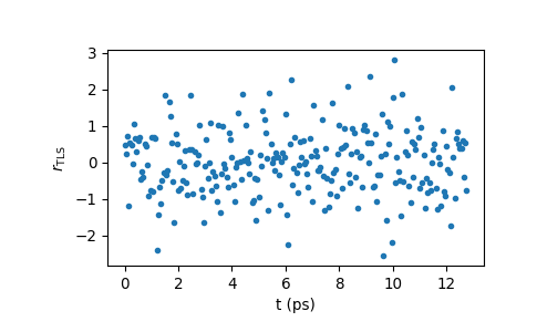
>>> _, ax = plt.subplots()
>>> ax.plot(t, result.r_tls, ".")
>>> ax.set_xlabel("t (ps)")
>>> ax.set_ylabel(r"$r_\mathrm{TLS}$")
>>> plt.show()