thztools.NoiseModel.noise_amp

method

NoiseModel.noise_amp(x, *, axis=-1)

Compute the time-domain noise amplitude.

Parameters:

xarray_like

Time-domain signal array.

axisint, optional

Signal axis. Default is the last axis in x.

Returns:

noise_amplitudendarray

Time-domain noise amplitude, in signal units.

Notes

For noise parameters \(\sigma_\alpha\), \(\sigma_\beta\), \(\sigma_\tau\) and signal vector \(\boldsymbol{\mu}\), the \(k\)-th element of the time-domain noise amplitude vector \(\boldsymbol{\sigma}\) is given by [1]

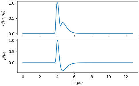
\[\sigma_k = \sqrt{\sigma_\alpha^2 + \sigma_\beta^2\mu_k^2 \ + \sigma_\tau^2(\mathbf{D}\boldsymbol{\mu})_k^2},\]

where \(\mathbf{D}\) is the time-domain derivative operator.

References

[1]

Laleh Mohtashemi, Paul Westlund, Derek G. Sahota, Graham B. Lea, Ian Bushfield, Payam Mousavi, and J. Steven Dodge, “Maximum- likelihood parameter estimation in terahertz time-domain spectroscopy,” Opt. Express 29, 4912-4926 (2021), https://doi.org/10.1364/OE.417724.

Examples

The following example shows the noise amplitude \(\sigma(t)\) for noise parameters \(\sigma_\alpha = 10^{-4}\), \(\sigma_\beta = 10^{-2}\), \(\sigma_\tau = 10^{-3}\) and the simulated signal \(\mu(t)\). The signal amplitude is normalized to its peak magnitude, \(\mu_0\). The noise amplitude is normalized to \(\sigma_\beta\mu_0\).

>>> import thztools as thz
>>> from matplotlib import pyplot as plt
>>> n, dt = 256, 0.05
>>> t = thz.timebase(n, dt=dt)
>>> mu = thz.wave(n, dt=dt)
>>> alpha, beta, tau = 1e-4, 1e-2, 1e-3
>>> noise_model = thz.NoiseModel(sigma_alpha=alpha, sigma_beta=beta,
... sigma_tau=tau, dt=dt)
>>> noise_amplitude = noise_model.noise_amp(mu)

>>> _, axs = plt.subplots(2, 1, sharex=True, layout="constrained")
>>> axs[0].plot(t, noise_amplitude / beta)
>>> axs[0].set_ylabel(r"$\sigma/(\sigma_\beta\mu_0)$")
>>> axs[1].plot(t, mu)
>>> axs[1].set_ylabel(r"$\mu/\mu_0$")
>>> axs[1].set_xlabel("t (ps)")
>>> plt.show()