Apply a frequency response function

Objects from thztools: apply_frf, timebase, wave.

from matplotlib import pyplot as plt
import numpy as np

import thztools as thz

Set the simulation parameters

n = 256  # Number of samples
dt = 0.05  # Sampling time [ps]
a = 0.5 # Scale factor
eta = 1.0 # Delay [ps]

Simulate an input waveform

t = thz.timebase(n, dt=dt)
mu = thz.wave(n, dt=dt)

Define the frequency response function

The frequency response function frfun rescales the input waveform by a and delays it by eta.

def frfun(omega, _a, _eta):
    return _a * np.exp(-1j * omega * _eta)

Apply the frequency response function

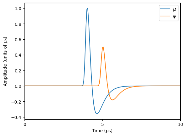
Generate the time-domain output waveform psi by applying frfun to mu with the apply_frf function.

psi = thz.apply_frf(frfun, mu, dt=dt, args=(a, eta))

Show the input and output waveforms

_, ax = plt.subplots()

ax.plot(t, mu, label=r'$\mu$')
ax.plot(t, psi, label=r'$\psi$')

ax.legend()

ax.set_xlabel('Time (ps)')
ax.set_ylabel(r'Amplitude (units of $\mu_{p})$')

ax.set_xticks(np.arange(0, 11, 5))
ax.set_xlim(0, 10)

plt.show()

Change sign convention

The above example uses the \(+i\omega t\) sign convention for representing harmonic waves with complex exponentials. NumPy also uses this convention in its definition of the FFT. Physicists commonly use the \(-i\omega t\) sign convention, which can cause confusion when translating between analytic expressions and computational expressions. The apply_frf function supports both sign conventions through the boolean parameter numpy_sign_convention.

def frfun_phys(omega, _a, _eta):
    return _a * np.exp(1j * omega * _eta)

psi_phys = thz.apply_frf(frfun_phys, mu, dt=dt, args=(a, eta), numpy_sign_convention=False)

_, ax = plt.subplots()

ax.plot(t, mu, label=r'$\mu$')
ax.plot(t, psi_phys, label=r'$\psi$')

ax.legend()

ax.set_xlabel('Time (ps)')
ax.set_ylabel(r'Amplitude (units of $\mu_{p})$')

ax.set_xticks(np.arange(0, 11, 5))
ax.set_xlim(0, 10)

plt.show()